In this post, you will learn how to repeat certain analysis using R and RMarkdown.

Recently, I saw many dissertations on higher education fundraising in which the researchers had used a data set, selected some variables, ran correlation or association as well as significance tests, and built a logistic regression model on the selected variables. The unfortunate part was that the researchers concluded based on weak results.

Almost every dissertation had the same approach. I was confident that this part can be programmed with a template using RMarkdown and RStudio. Since repeating this type of analysis is hardly special, I hope that future researchers will focus on bigger problems.

Let’s go through the steps to create this document.

R Markdown Document

We will open a New R Markdown document and use Tufte Handout template. Make sure that this works on your computer before you make any changes. If you get errors, you will have to update some settings or install other packages.

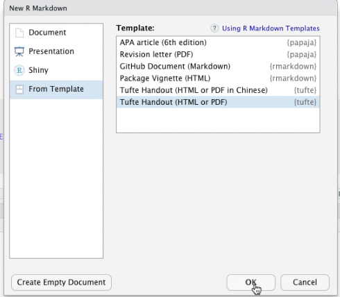
Once you know that the document knits, get rid of all other stuff below the Introduction header.

Then make changes in the header such as the title and author.

Also replace the output format with tufte_book2.

Replace the bibliography file name, which I named repeat-analysis.bib

R Code

Insert a R chunk to load our favorite libraries and custom functions. Here, I have a mode function (copied from Stackoverflow, of course), which we will use to replace missing values.

```{r libsfunctions, include=FALSE}
library(readr)

library(dplyr)
library(purrr)
library(tables)
library(janitor)
library(vcd)
library(scales)
library(kableExtra)
library(stringr)

Mode <- function(x) {
  x <- x[!is.na(x)]
  ux <- unique(x)
  ux[which.max(tabulate(match(x, ux)))]
}
```
Code language: R (r)

Next, we will load and manipulate a dataset. This synthetic data set is from my and Rodger Devine’s book Data Science for Fundraising.

Let’s see the data manipulation step by step.

```{r loaddata, include=FALSE}
sample_data <- read_csv("https://www.dropbox.com/s/ntd5tbhr7fxmrr4/DonorSampleDataCleaned.csv?dl=1")

sample_data_refi <- sample_data %>%
  filter(ALUMNUS_IND == 'Y') %>%
  select(
    ID,
    AGE,
    MARITAL_STATUS,
    GENDER,
    PARENT_IND,
    HAS_INVOLVEMENT_IND,
    WEALTH_RATING,
    DEGREE_LEVEL,
    PREF_ADDRESS_TYPE,
    EMAIL_PRESENT_IND,
    TotalGiving
  ) %>%
  mutate(TotalGivingGroup = cut(
    TotalGiving,
    breaks = c(0, 100, 1000, 10000, max(TotalGiving)),
    include.lowest = T,
    labels = c("0-100", "101-1000", "1001-10000", "10000+")
  )) %>%
  mutate(AgeGroup = cut(
    AGE,
    breaks = c(0, 35, 60, 10000),
    include.lowest = T,
    labels = c("0-35", "36-60", "60+")
  )) %>%
  mutate(ON_CAMPUS_RESIDENCE = sample(c("Y", "N"), size = nrow(.), replace = TRUE)) %>%
  mutate(EVENT_ATTEND_IND = sample(c("Y", "N"), size = nrow(.), replace = TRUE)) %>%
  mutate(DISTANCE_FROM_CAMPUS = sample(
    c("0-50 miles", "51-100 miles", "100+ miles"),
    size = nrow(.),
    replace = TRUE
  )) %>%
  mutate_if(is.numeric, list( ~ replace(., is.na(.), median(., na.rm = TRUE)))) %>%
  mutate_if(is.character, list( ~ replace(., is.na(.), Mode(.))))

names(sample_data_refi) <- gsub("_", " ", names(sample_data_refi))
```
Code language: R (r)

First, I removed any non-alumni from the dataset. Line # 5.

Then, I selected a few variables of importance. Lines # 6-18.

Then I created buckets using the Total Giving variable. Lines # 6-18.

Same with the Age variable. Lines # 25-30.

I added a few fake variables and randomly generated their values. Lines # 31-37.

Finally, I replaced the missing values from a numeric variable with the median of that variable and for a character variable, I used Mode value of that variable. Lines # 38-39.

I also replaced the underscores in the variable names with spaces. Line # 41

Map Functions

Before we generate statistical results, let’s take a detour to understand the map functions from the package purr.

The map function is similar to the apply family of functions in that you can apply any function to a list and do something with the results. In our case, we want to apply statistical tests to each variable in our dataset.

Let’s take a simple example. We have two variables in our data frame x and y. We want to find the mean of each of those variables. Of course, this can be done running summary(), but we want to see how we can this function for complex use cases.

library(dplyr)
library(purrr)

data.frame(x = 1:10, y = 11:20) %>% 
  summary()
Code language: R (r)

Here’s using the map function. The tilde sign here represents the data that’s before the map command.

And .x represents each column from the previous data set.

data.frame(x = 1:10, y = 11:20) %>% 
  map(~ mean(.x)) %>% 
  str()
Code language: R (r)

When we execute this, we can a list of two items, one for each variable as seen by the str function.

Instead of getting a list, we can return a dataframe using map_dfr function.

data.frame(x = 1:10, y = 11:20) %>% 
  map(~ mean(.x)) %>% 
  map_dfr(~ broom::tidy(.), .id = 'source')
Code language: PHP (php)

Or, we can use a shortcut function map_dbl to return a vector with the mean values.

data.frame(x = 1:10, y = 11:20) %>% 
  map_dbl(~ mean(.x))
Code language: R (r)

Let’s run a linear regression model on variables from a dataset.

First, let’s create a test data frame with our dependent variable, z, takes some function form of x and y.

test_df <- data.frame(x = 1:10, y = 11:20) %>% 
  mutate(z = (x+y)^2)  
Code language: R (r)

To do so, we exclude z from the data set that’s fed to the map function, but provide the original dataset to the data argument of the map function.

select(test_df, -z) %>% 
  map( ~ lm(z ~ .x, data = test_df))
Code language: R (r)

We get a list with two models for x and y each.

Let’s extract the summary for each of the models.

select(test_df, -z)  %>% 
  map( ~ lm(z ~ .x, data = test_df)) %>% 
  map(summary)
Code language: R (r)

Now, let’s extract the R-square statistic from each model.

select(test_df, -z)  %>% 
  map( ~ lm(z ~ .x, data = test_df)) %>% 
  map(summary) %>% 
  map_dbl("r.squared")
Code language: R (r)

If we want to get all the summary statistics, we can use the tidy function from the broom package and return these as a dataframe.

select(test_df, -z)  %>% 
  map( ~ lm(z ~ .x, data = test_df)) %>% 
  map_dfr(~ broom::tidy(.), .id = 'source') 
Code language: R (r)

This forms the backbone of our analysis.

We create data frames or lists containing the statistics we are interested in and then extract values for the variables we are interested in. For example, we want to extract the p-value of the y-variable, here’s how we can do so.

select(test_df, -z)  %>% 
  map( ~ lm(z ~ .x, data = test_df)) %>% 
  map_dfr(~ broom::tidy(.), .id = 'source') %>% 
  filter(source == 'y', term == '.x') %>% 
  select(p.value) %>% 
  as.double
Code language: R (r)

Statistical Analysis

Following the map function approach, let’s run statistical analysis and store them. Insert a new R chunk and enter the following code.

First, let’s run the analysis of variance on each of the nominal variable and the Total Giving Group variable. Then extract the p-value for each of those variables.

aov_values <- sample_data_refi %>% 
  select(-TotalGivingGroup, -ID, -TotalGiving, -AgeGroup) %>% 
  select_if(is.character) %>% 
  map(~ aov(TotalGiving ~ .x, data = sample_data_refi)) %>%
  map_dfr(~ broom::tidy(.), .id = 'source') %>%
  mutate(p.value = round(p.value, 8))
Code language: R (r)

Next, get the Pearson’s product moment correlation coefficient for numeric variables.

pearson_values <- sample_data_refi %>% 
  select(-TotalGivingGroup, -ID, -TotalGiving, -AgeGroup) %>%
  select_if(is.numeric) %>% 
  map(~ cor.test(sample_data_refi$TotalGiving, .x,  method = "pearson")) %>%
  map_dfr(~ broom::tidy(.), .id = 'source') %>%
  mutate(p.value = round(p.value, 8))
Code language: R (r)

Then Cramer’s V value to measure the association between Total Giving group variable and each nominal variable.

cramer_values <- sample_data_refi %>%
  select(-ID, -TotalGiving, -AGE, -TotalGivingGroup) %>%
  map(~ xtabs(~TotalGivingGroup + .x, data = sample_data_refi)) %>% 
  map(assocstats) %>% 
  map_dbl("cramer")
Code language: R (r)

Now, let’s build logistic regression models for each of the variables and the Total Giving group variable.

logistic_reg_stats <- sample_data_refi %>%
  select(-ID, -TotalGiving, -AGE, -TotalGivingGroup) %>%
  map(~ glm(TotalGivingGroup ~  .x, data = sample_data_refi, family = binomial)) %>% 
  map_dfr(~ broom::tidy(.), .id = 'source')  %>% 
  mutate(term = gsub(pattern = ".x",replacement =  "", x = term))
Code language: R (r)

And extract, the AIC value of these models.

logistic_reg_aic <- sample_data_refi %>%
  select(-ID, -TotalGiving, -AGE, -TotalGivingGroup) %>%
  map(~ glm(TotalGivingGroup ~  .x, data = sample_data_refi, family = binomial)) %>% 
  map_dbl("aic") 
Code language: R (r)

Now, we have all the results we need to put them into a nice-looking document.

Generate Markdown Syntax

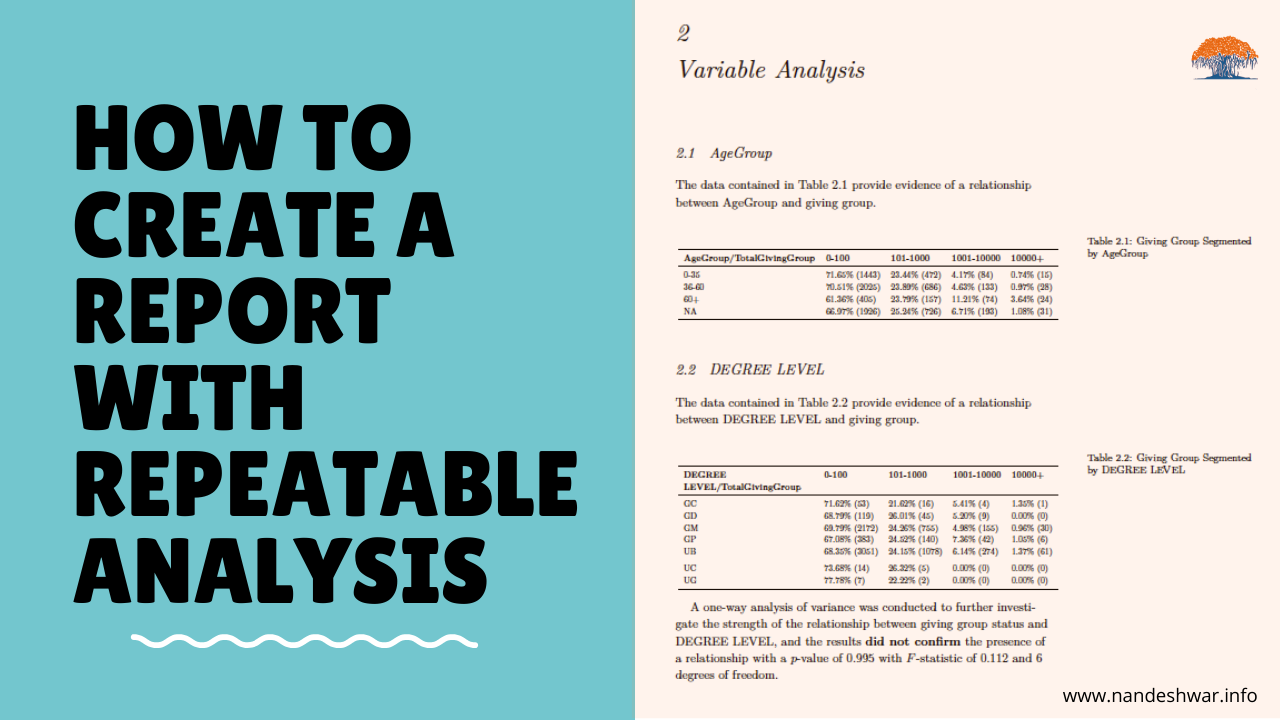
Let’s add some text to the introduction section and create a new section called Variable analysis.

We will now insert a R chunk to create sections for each variable. In this section, we will report the proportions and counts for each value in the variable. We will then generate a conditional sentence based on the p-value from the ANOVA results.

vars_to_study <-
  sort(names(
    select(sample_data_refi, -ID, -TotalGiving, -TotalGivingGroup, -AGE)
  ))

for (var in vars_to_study) {
  cat(paste("##", var, "\n"))
  
  cat(
    paste(
      "The data contained in Table",
      str_replace_all(paste0("\\@ref(", "tab:proptable", var, ")"), " ", ""),
      "provide evidence of a relationship between",
      var,
      "and giving group."
    )
  )
  
  cat("\n\n\n")
  
  fi_df <- select(sample_data_refi, TotalGivingGroup)
  prnt_tbl <- sample_data_refi %>%
    tabyl(!!sym(var), TotalGivingGroup)  %>%
    adorn_percentages("row") %>%
    adorn_pct_formatting(rounding = "half up", digits = 2) %>%
    adorn_ns() %>%
    adorn_title("combined")
  
  
  kable_cmd <- knitr::kable(
    prnt_tbl,
    format = "latex",
    label = paste0("proptable", gsub(" ", "", var)),
    caption = paste0("Giving Group Segmented by ", var),
    booktabs = TRUE
  ) %>%
    row_spec(0, bold = TRUE) %>%
    column_spec(1, width = "15em") %>%
    kable_styling(latex_options = "scale_down")
  
  print(kable_cmd)
  
  cat("\n\n\n")
  
  
  aov_df <- filter(aov_values, source  == var, term == ".x")
  
  pearson_df <- filter(pearson_values, source == var)
  
  if (nrow(aov_df) == 1) {
    prnt_txt <-
      paste(
        "A one-way analysis of variance was conducted to further investigate the strength of the relationship between giving group status and",
        var
      )
    
    prnt_txt <-
      paste0(
        prnt_txt,
        ", and the results **",
        ifelse(aov_df$p.value <= 0.05, "confirmed", "did not confirm"),
        "** the presence of a relationship with a $p$-value of ",
        round(aov_df$p.value, 3)
      )
    
    
    prnt_txt <-
      paste(
        prnt_txt,
        " with $F$-statistic of",
        round(aov_df$statistic, 3),
        "and",
        aov_df$df,
        "degrees of freedom."
      )
    
    cat(prnt_txt)
  }
  
  cat("\n\n")
}
Code language: R (r)

First, we create a loop to go through the variables we want to report on. Line # 6.

We then create a markdown subsection for that variable. Line # 7.

We write a generic sentence to provide a reference to the proportions table. Lines # 9-17.

We create the proportions table using the tabyl function from the janitor package. You will see that I am using two exclamation marks and sym function to get the underlying column name from the looping variable. Lines # 22-27.

We use the adorn functions to add percentages and totals.

Then using the kable function and some functions from the kableExtra package we create a proportions table to our liking. Lines # 30-39.

We have to add a few newline characters to make sure our final results look good.

Next, using the p-values from the ANOVA results, we write a conditional sentence i.e. if the p-value is less than or equal to 0.05, there is a relationship between that variable and the total giving variable. Lines # 57-64.

We have to add a few newline characters to make sure our final results look good.

Logistic Regression Results

Now, we report out the results from the logistic regression models.

We create a new section.

We pull the important variables using the p-value again. For example’s sake, I am using 0.5 p-value as a threshold.

imp_vars <- filter(aov_values,  term == ".x", p.value <= 0.5) %>% 
  .$source
Code language: R (r)

Using an inline R command, we print all the important variables.

In a new R chunk, we follow the same approach from the previous loop.

for (var in imp_vars) {
  cat(paste("##", var, "\n"))
  
  cat(
    paste(
      "The data in Table",
      str_replace_all(paste0(
        "\\@ref(", "tab:logregresultstable", var, ")"
      ), " ", ""),
      "show the logistic model using",
      var,
      " as an independent variable and the giving group as a dependent variable."
    )
  )
  
  cat("\n\n\n")
  
  prnt_df <-
    filter(logistic_reg_stats, source == !!var) %>% select(-source)
  
  kable_cmd <- knitr::kable(
    prnt_df,
    format = "latex",
    label = paste0("logregresultstable", gsub(" ", "", var)),
    caption = paste0("Logistic Regression Results for ", var),
    booktabs = TRUE
  ) %>%
    row_spec(0, bold = TRUE) %>%
    kable_styling(latex_options = "scale_down")
  
  
  print(kable_cmd)
  
  
  cat("\n\n\n")
  
  
  prnt_txt <-
    paste0(
      "A correlation analysis using Cramer's V was conducted to further investigate the association between giving level groups and ",
      var,
      " and the value was found to be ",
      round(cramer_values[var], 4),
      ", which indicates a **",
      ifelse(cramer_values[var] >= 0.5, "strong", "weak"),
      "** association",
      "."
    )
  
  prnt_txt <-   paste0(
    prnt_txt,
    " The logistic regression generated AIC value for ",
    var,
    " was ",
    comma(logistic_reg_aic[var]),
    "."
  )
  
  cat(prnt_txt)
  
  cat("\n\n")
}
Code language: R (r)

We create a new subsection.

We print a generic sentence referencing the results from the logistic regression model. Lines #4-14.

Then select the appropriate rows from the logistic regression results data frame and print the table. Lines #18-29.

We add conditional text based on the Cramer’s V values whether the association was strong or weak. Lines #39-48.

And finally, we print the AIC values from the logistic regression model. Lines #50-57.

We have everything to create our final document. Let’s hit the “knit” button to see the document.

There it is. A beautiful document with descriptive statistics, vague inferences, and dubious predictive models.

Conclusion

This could be a good starting point for anyone who wants to analyze his or her data. But this type of analysis should not form the core components of a dissertation, especially when the scientific journals are discouraging or banning the null hypothesis significance testing to draw inferences. As the editor of the Basic and Applied Social Psychology journal said, “p < .05 bar is too easy to pass and sometimes serves as an excuse for lower quality research.”

p < .05 bar is too easy to pass and sometimes serves as an excuse for lower quality research

Editor, Basic and Applied Social Psychology Journal

I hope that you learned how to automate and repeat statistical analysis using R and Rmarkdown.

Video

Some Books You May Like

Table could not be displayed.

Last update on 2022-05-05 / Affiliate links / Images from Amazon Product Advertising API